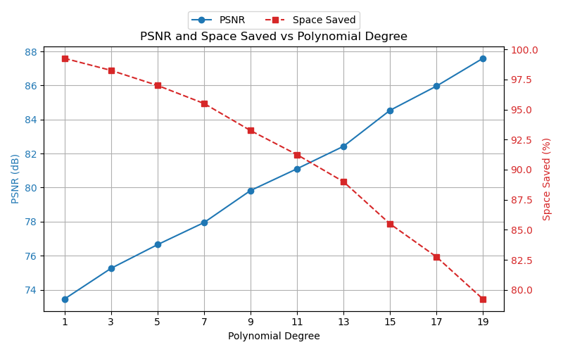
Now we take a look at the metrics, and how they vary with polynomial degree. This can be altered to use a different metric, and is not limited to PSNR.

import sys
import os

# Add project root to path
sys.path.append(os.path.abspath(".."))

import numpy as np
import imageio.v3 as iio
import matplotlib.pyplot as plt

from core.data import CompressionMetrics
from core.utils import convert_to_gray_scale
from core.image import compress_image, reconstruct_image

img_rgb = iio.imread("../sources/garden_table.png").astype(np.float32)
img_gray = convert_to_gray_scale(img_rgb)

# Hyperparameters
lp_degree = 0.5
block_size = 20
cutoff = None
poly_degrees = np.arange(2, 22, 2) - 1

metrics_list = []
img_gray_rec_list = []
for poly_degree in poly_degrees:
    c, X_design, rescale = compress_image(
        image=img_gray,
        poly_degree=poly_degree,
        block_size=block_size,
        lp_degree=lp_degree,
        lasso=False,
        cutoff=cutoff
    )
    img_gray_rec = reconstruct_image(c, X_design, rescale)
    metrics_list.append(CompressionMetrics(img_gray, img_gray_rec, c))
    img_gray_rec_list.append(img_gray_rec)

# Extract values
psnr_values = [m.psnr for m in metrics_list]
space_saved_values = [m.space_saved for m in metrics_list]

Plotting PSNR (dB) vs Polynomial Degree

# Create figure and primary axis
fig, ax1 = plt.subplots(figsize=(8, 5))

# Plot PSNR on primary y-axis
ln1 = ax1.plot(poly_degrees, psnr_values, marker="o", linestyle="-", color="tab:blue", label="PSNR")
ax1.set_xlabel("Polynomial Degree")
ax1.set_ylabel("PSNR (dB)", color="tab:blue")
ax1.tick_params(axis="y", labelcolor="tab:blue")
ax1.grid(True)
ax1.set_xticks(poly_degrees)

# Plot space saved on secondary y-axis
ax2 = ax1.twinx()
ln2 = ax2.plot(poly_degrees, space_saved_values, marker="s", linestyle="--", color="tab:red", label="Space Saved")
ax2.set_ylabel("Space Saved (%)", color="tab:red")
ax2.tick_params(axis="y", labelcolor="tab:red")

# Combine legends and place outside top-left
lines = ln1 + ln2
labels = [l.get_label() for l in lines]
ax1.legend(lines, labels, loc="upper center", bbox_to_anchor=(0.5, 1.15), ncol=2)

plt.title("PSNR and Space Saved vs Polynomial Degree")
plt.tight_layout()
plt.savefig("../results/image/garden_table/plots/psnr__pinv__bs=%s__cutoff=%s__lp=%s__pd=%s-%s.png" % (block_size, cutoff, lp_degree, poly_degrees[0], poly_degrees[9]))
plt.show()

image_psnr

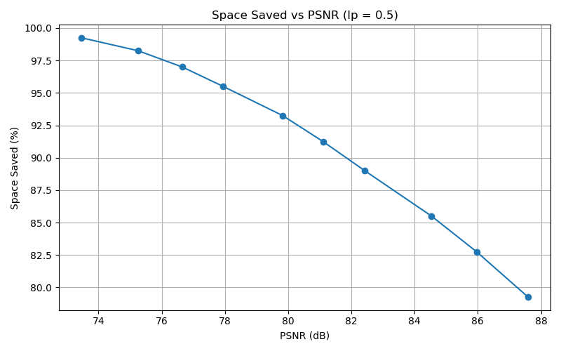
Plotting Space Saved (%) vs Plotting PSNR (dB)

# Create figure and primary axis
fig, ax = plt.subplots(figsize=(8, 5))

# Plot PSNR vs space saved
ax.plot(psnr_values, space_saved_values, marker="o", linestyle="-")
ax.set_xlabel("PSNR (dB)")
ax.set_ylabel("Space Saved (%)")
ax.grid(True)


plt.title("Space Saved vs PSNR (lp = %s)" % lp_degree)
plt.tight_layout()
plt.savefig("../results/image/garden_table/plots/space__vs__psnr__pinv__bs=%s__cutoff=%s__lp=%s__poly_deg=%s-%s.png" % (block_size, cutoff, lp_degree, poly_degrees[0], poly_degrees[9]))
plt.show()

image_space_vs_psnr

Let’s take a look at some of the images, to see how well it’s working

plt.imshow(img_gray_rec_list[0], cmap="gray")
# plt.savefig("results/garden_table/image-gray__pinv__bs=%s__cutoff=%s__lp=%s__poly_deg=%s.png" % (block_size, cutoff, lp_degree, poly_degrees[0]))
plt.show()

plt.imshow(img_gray_rec_list[5], cmap="gray")
# plt.savefig("results/garden_table/image-gray__pinv__bs=%s__cutoff=%s__lp=%s__poly_deg=%s.png" % (block_size, cutoff, lp_degree, poly_degrees[5]))
plt.show()

plt.imshow(img_gray_rec_list[9], cmap="gray")
# plt.savefig("results/garden_table/image-gray__pinv__bs=%s__cutoff=%s__lp=%s__poly_deg=%s.png" % (block_size, cutoff, lp_degree, poly_degrees[9]))
plt.show()

Depending on the parameters you chose, you may see why it’s important to verify that the quality of the reconstructed images matches their respective metrics. In some cases, we observed a much higher PSNR, but either the quality was poor, or artifacts were clearly visible. Sometimes we experienced both. Similarly, the quality may be decent, or even excellent, but the PSNR is low.

Side note: To save any/all images and/or figures, uncomment the plt.savefig and/or np.save line (if not already uncommented), and adjust the path to your desired path. If you decide to alter the naming convension, it’s best to ensure that it remain consistent throughout the project.

Back to Home

<- Previous

Next ->

This site is open source. Improve this page.

lp-compression